Chap 5. Neural Network

5.1 Neuron Model

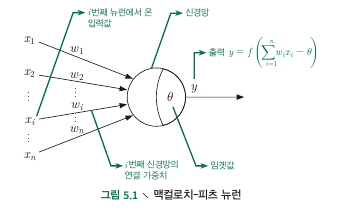
M-P Neuron model

Input : receive input signals from $n$ neurons
Process : weighted sum of received signals is compared against the threshold
Output : signal produced by activation function i.e.) $\text{output = } f({\bf w^T x + b})$

Activation function

Unit step function (양수이면 1, 음수이면 0)
sigmoid function ($\sigma(x) = \frac{1}{1+e^{-x}}$) : unit step function은 미분불가능성, 불연속성 등의 좋지 않은 조건으로 인해 sigmoid를 사용.
$(-\infty, +\infty)$의 값을 $[0,1]$로 밀어넣을 수 있으므로 squashing function이라 불리기도 한다.

5.2 Perceptron and Multi-layer Networks

Perceptron : 2개 layer (input, output)으로 구성, input layer는 input을 받아서 output layer에 전달, output layer는 M-P neuron으로 threshold 연산 수행.

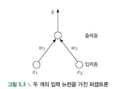
Perceptron으로 Logic Gate를 구현 가능 (AND, OR, NAND) : by tuning $w_1, w_2, \theta$
Activation function을 USF로 가정하면,
AND : $w_1, w_2 = 1, \theta = 2$ : if $x_1, x_2$ are all 1, then output is 1
OR : $w_1 = 1, w_2 = 1, \theta = 0.5$: if one of $x_1, x_2$$is 1, then output is 1
NOT : $w_1 = -0.6, w_2 = 0, \theta = -0.5$ : if $x_1$ is 1, then output is 0, else otherwise

Perceptron learning

weight $w_i$ and threshold $\theta$ can be learned from training data
threshold를 상수에 대한 weight로 보면 모든 learning process를 weight에 대한 update로 생각할 수 있음.

\[\begin{aligned} w_i &\leftarrow w_i + \Delta w_i \\ \Delta w_i &= \eta (y-\hat y) x_i \\ \eta \in (0,1) &\text{: Learning rate} \end{aligned}\]

(Single layer) Perceptron은 Linearly seperable problem에 대한 학습만이 가능. if XOR (00, 11 = 0, 01,11=1) 같은 회로는 하나의 선으로 분류가 불가능하므로 학습이 안됨 (but it is guaranteed to converge for linear seperable ploblems)
제한적 학습 능력

Multi-layer perceptrons

Hidden layer : Activation function이 적용되는 input layer와 output layer 사이의 layer.
Linear seperable problem이 아닌 경우에도 문제 해결이 가능.

5.3 Error Backpropagation Algorithm

BP (error Back Propagation)
Constraints(Datas)

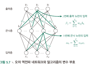
\[\begin{aligned} \text{Given dataset } D &= \{({\bf x_i}, y_i)\}, {\bf x_i}\in R^d, y_i \in R^l\ (i=1,2,\cdots, m) \\ \theta_j &\text{ : threshold of the jth output neuron} \\ \gamma_h &\text{ : threshold of the hth hidden neuron} \\ v_{ih} &\text{ : connection weight btw input - hidden} \\ w_{hj} &\text{ : connection weight btw hidden - output} \end{aligned}\]

Consider a single sample $\bf x_i$ to be trained at Multi-layered network with 1 hidden layer
Hidden Layer의 output $b_i$ :

\[\begin{aligned} b_i &= f(\alpha_h - \gamma_h) \\ \alpha_h &= \sum_{i=1}^d v_{ih} x_i \end{aligned}\]

Ouptut layer의 output $\hat y_j^k$ :

\[\begin{aligned} \hat y_j ^k &= f(\beta_j -\theta_j) \\ \beta_j &= \sum_{i=1}^q w_{hj}b_h\end{aligned}\]

Data index $k$, ($\bf x_k$) 에 대한 sum of squared(?) error :

\[E_k = \frac{1}{2} \sum_{j=1}^l (\hat y_j^k - y_j^k)^2\]

Parameters to tune : $v_{ih}, w_{hj}, \theta_j, \gamma_h$
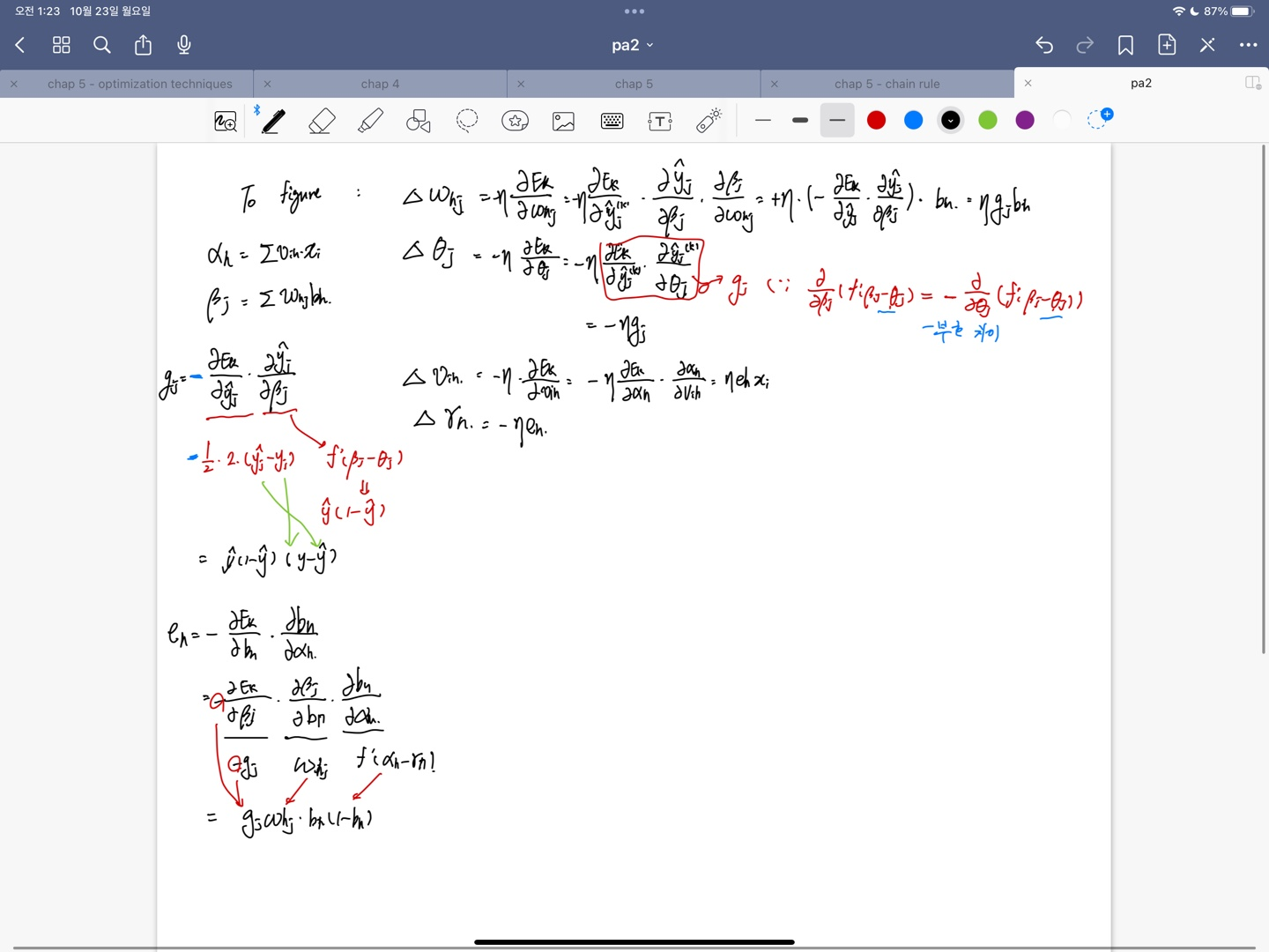
How to tune : update $v$ with delta v

\[\Delta w_hj = -\eta \frac{\partial E_k}{\partial w_hj}\]

각 변수에 대한 Delta는 $E_k$를 object function으로 보고 $E_k$를 내가 tune 하고자 하는 변수에 대한 편미분을 한 다음 학습률 $\eta$와 -1을 곱한 값으로 Delta를 정하여 업데이트 한다. (기울기는 증가하는 방향이 아니라 줄어드는 방향쪽으로 찾아야 Minimum을 찾으니까 -를 붙임.) 이 때 계산은 계산 순서에 따라 chain rule을 적용,
object function에는 sigmoid function을 사용했다고 가정. $\hat y_j^k$나, hidden layer의 output을 미분할 때에는 weighted sum이 아닌, function안에 weighted sum이 들어간 형태를 사용하게 되므로 function 자체의 derivative를 취해주는 과정, 속미분 과정 잊지말아야.
Derivation process

Accumulated BP Algorithm

minimizes the accumulated error on the whole training set

\[E = \frac{1}{m} \sum_{k=1}^m E_k\]

Tunes parameter less frequently.
은닉층 뉴런 개수는 trial-and-error밖에 없음

How to overcome OVERFITTING

Early stopping : training error 감소, validation error 증가하는 순간 terminate
Regularization : recall tikhonov regulatization (also minimizes the squared sum of weights)

5.4 Global / Local minimum

find $\bf w^\ast, \theta^\ast$ s.t. gradient of E is zero : local minimum
항상 local minimum이 1개(local=global)임이 보장되지는 않음

How to “jump out” from the local minimum

Simulated annealing (담금질 기법) : 일정활률로 현재 해보다 나쁜 결과로 이동. (차선의 해를 받을 확률이 점점 줄어들게 되면서, 시간에 따라 algorithm이 안정)
Stochastic gradient descent : 기울기 계산시 랜덤요소를 추가하여, local minimum에서 계산값이 0이 아닐 수도 있음.
Genetic algorithm : 비슷..

5.5 Other common neural networks

NOT considered in this lecture

5.6 Deep learning

NOT considered in this lecture

댓글을 불러오는 중입니다.