Disclaimer

📣 본 포스트는 조우쯔화의 단단한 머신러닝 책을 요약 정리한 글입니다.

Chap 4. Decision tree

4.1 Basic process

• Decision Tree Learning algorithm
• Input : Testing set $D$, Feature set $A$

Process :

1. generate node $i$
2. if $\forall D \in C$ :
   • Mark node $i$ as a class $C$ leaf node, return
3. if $A=\varnothing \ \text{or} \ \forall D $ take some value on $A$ :
   • Mark node $i$ as a leaf node, label = majority class in $D$, return
4. Set optimal splitting feature $a^*$ from $A$ (Entropy, GINI, etc…)
5. for each value $a_{}^{v}$ in $a_{}$, do :
   1. Generate branch for node $i$ ; $D_v$ is subset of samples taking $a_{}^{v} \text{on } a_{}$
   2. if $D_v$ is empty :
      • Mark $D_v$ as leaf node, label it with majority class in $D$, return
   3. else :
      • $D_v$ = self($D_v$, $A \ \backslash \ {a_*}$)

Output : Decision tree with root node $i$

4.2 Split selection

Split by information entropy

• Information Entropy (or simply entropy)

\[\begin{aligned}Ent(D) = -\sum_{k=1}^{f} p_k \log_2 p_k \end{aligned}\]

• $f$ : Number of features
• Entropy 의미 : 클 수록 잘 분배되어 있는 것. 0에 가까울 수록 한쪽으로 편향되어 있다는 뜻 (작을 수록 순도가 높음)
• Gain of splitting samples by feature

\[Gain(D, feature) = Ent(D)-\sum_{k=1}^{V}\frac{\vert D^v\vert}{\vert D \vert} Ent(D^v)\]

• 모든 남아있는 feature에 대한 information gain을 계산하여 가장 gain이 높은 (엔트로피를 효과적으로 줄일 수 있는) feature를 택하여 분할을 진행

Split by gain ratio

• Gain ratio : Gain 자체가 커지게 하려면 attribute의 수가 많은 feature가 유리하게 작동함. 즉 이에 대한 보정을 하는 것이 gain ratio 보정(?)

\[\begin{aligned} \text{Gain ratio} \ (D, a) =& \ \frac{Gain(D,a)}{IV(a)} \\ IV(a) =& \ -\sum_{k=1}^{V} \frac{\vert D^v\vert}{\vert D \vert} \log_2 \frac{\vert D^v\vert}{\vert D \vert} \end{aligned}\]

• Gain ratio is biased towards features with fewer possible values : possible values 수가 많은 경우 (like case of ID) 저평가함.

Split by GINI Index

• Gini(D) : 임의의 2개 sample이 서로 다른 클래스일 확률. (Gini(D)가 클 수록 D의 purity는 높음)

\[\begin{aligned}Gini(D) =& \ \sum_{k=1}^{N(attr)}\sum_{k'\neq k}p_k p_{k'} \\ =& \ 1-\sum_{k=1}^{N(attr)}p_k^2 \end{aligned}\]

• Gini index가 가장 작은 feature를 고름

\[\text{Gini index}(D,a) = \sum_{v=1}^V \frac{\vert D^v\vert}{\vert D \vert} Gini(D^v)\]

4.3 Pruning

• Deal with overfitting.
• General strategies : pre/post-pruning
• First, using hold-out method, split dataset into training and validation set

Pre-pruning

• comparing before/after splitting
• 가지치기를 하기 전에 splitting 과정에서부터 pre-pruning을 진행하는 것.
• validation set에 대한 accruacy를 splitting 전후로 계산, 그 rate가 늘어나지 않으면 prune, 그렇지 않으면 split
• Advantages : Reduce the risk of overfitting, computational cost of training and testing
• Disadvantages : Risk of underfitting

Post-pruning

• 이미 만들어진 decision tree에 대한 ‘post’ pruning
• 먼저 total tree에 대한 accruacy를 계산.
• 하위 node부터, pruning 전후의 accuracy 차이를 계산, 효용이 있다면 pruning 진행. (같다면 진행 x)
• Advantages : less prone to underfitting -> better generalization ability
• Disadvantages : training time of post-pruning is much longer (하위노드부터 하나씩 전부 따져봐야 하므로)

4.4 Continuous values & missing values

Continuous values

• Discetization Stretagy (Bi-partition) : Dataset D에서 feature a에 대해 t를 기준으로 2개의 group으로 나눔.
• 이 때 Split point의 후보 분할점이 되는 점

\[T_a = \{\frac{a^i+a^{i+1}}{2}\} \text{ for 1 }\leq i \leq n-1\]

• Midpoint $T_a$가 사용되며, 이를 이용해 구한 Gain은 다음과 같음.

\[\begin{aligned}Gain(D,a) =& \ \max_{t\in T_a} Gain(D,a,t) \\ =& \ max\ Ent(D)-\sum_{\lambda\in\{-,+\}} \frac{\vert D_t^\lambda\vert}{\vert D\vert} Ent(D_t^\lambda)\end{aligned}\]

• a라는 property를 이용해 D를 분리할 때 t라는 새로운 변수까지 고려해서 gain이 최대화되는 t를 선택하겠다는 뜻.

Missing Values

• To solve problems :
  1. feature의 선택
  2. feature가 선택된 경우 샘플이 결측값이라면 어떻게 분할할 것인가.
• 특정 feature $a$에 대하여:
  • $w_x$ : weight for sample $x$
  • $D$ : total data
  • $\tilde D$ : data that has values of $a$
  • $\tilde D_k$ : $k$th sample(classifier’s ground truth)
• $\rho$ : 전체 Data 중 $a$의 데이터가 존재하는 비율 (weighted)

\[\rho = \frac{\sum_{x\in \tilde D} w_x}{\sum_{x\in D} w_x}\]

• $\tilde p_k$ : 결측값 없는 데이터 중 label : $k$의 비율 (weighted)

\[\tilde p_k = \frac{\sum_{x\in \tilde D_k} w_x}{\sum_{x\in \tilde D} w_x}\]

• $\tilde r_v$ : 결측값 없는 데이터 중 feature $a$에 대해서 $v$의 값을 갖는 비율 (weighted)

\[\tilde r_v = \frac{\sum_{x\in \tilde D^v} w_x}{\sum_{x\in \tilde D} w_x}\]

• Gain, Entropy의 재정의

\[\begin{aligned}Gain(D,a) =& \ \rho \times Gain(\tilde D, a) \\ =& \ \rho \times \bigg(Ent(\tilde D) - \sum_{v=1}^V \tilde r_v Ent(\tilde D^v)\bigg) \\ Ent(\tilde D) =& \ -\sum_{k=1}^{N(attr)} \tilde p_k \log_2\tilde p_k \end{aligned}\]

• 만약 feature $a$로 분할 했는데 특정 sample $x$의 feature $a$가 결측값이라면, $x$를 모든 하위 node에 동일하게 귀속시키는 대신 그 가중치(weight)을 $w_x$에서 $\tilde r_v w_x$로 update한다.

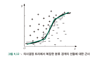
4.5 Multivariate Decision Trees

• Feature axis에 data point를 plot 하였을 때 Decision tree가 하는 일은 axis에 parallel한 경계선을 긋는 행위.
• Parallel하지 않은 대각선 line을 그릴 수 있다면?