
[제어공학개론] Lec 18 - Discrete time domain system
📢Precaution
본 게시글은 서울대학교 심형보 교수님의 23-2 제어공학개론 수업 내용을 바탕으로 작성되었습니다.
Discrete - Time domain system
Physical world는 analog이지만, Cyber world는 컴퓨터로 진행되므로, 일정한 시간 간격마다 system clock에 따라 sampling되고 결과가 출력됨.
Cyber world와 Physical world를 이어주는 2개의 선에서, Controller output 을 $P(s)$에 전달해주는 Actuator, 혹은 Digital to Analog Convert(DAC). 그리고 $P(s)$의 출력 $y$를 Sampler (Analog to Digtal Converter) (Switch형태로 표시) 가 있음.
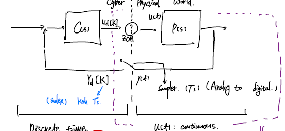
Sampling time $T_s$에 대해서 Discrete signal을 $y_d[K]$의 형태로 index로 적음.
Discrete signal에는 $ y, t $ 2개에 대해 discrete할 수 있는데, 일단 여기서는 $t$가 discrete한 경우만 다룸.
그렇다면 Physical system 또한 $z$-transform에 의해 일종의 input-output이 있는 system으로 볼 수 있음.
$u_d[K]$가 input, $P_d[Z]$의 transfer function을 가지고, $y_d[K]$가 출력.
ZOH (Zero-order holder) :
Converter :
\[u(t) = u_d[K] \text{ for }KT_s\leq t \leq (K+1)T_s\]State-space representation of discrete system
Differential이 아닌 Difference(차분) equation이라고 불림
\[\begin{aligned}\bar{x}[K+1] &= \bar{A} \bar{x}[K] + \bar{B} \bar{u}[K] + W[K] \\\bar{y}[K] &= \bar{C} \bar{x}[K] + \bar{D} \bar{u}[K]\end{aligned}\]일종의 MDP(Markov decision process)
stochastic하게 만들기 위해 $W[K]$ 라는 랜덤확률변수를 도입하기도 함. (ML에서)
물리적 실체인 원래의 A, B, C, D 시스템으로부터 Sampling한 것이라고 볼 수 있음. (물론 컴퓨터에서 만들어진 system일 경우 애초에 실체가 discrete일수도)
recall the Variation of Constant Formula
\[\begin{aligned}x(t) &= x(0) e^{At} + \int_0^t e^{A(t-\tau)} B u(\tau) \, d\tau \\\bar{x}[1] &= x(T_s) = e^{A T_s} x[0] + \int_0^{T_s} e^{A(T_s - s)} B u(s) \, ds\end{aligned}\]when using ZOH, $u(s)$ is constant for one period.
\[\begin{aligned}\bar{x}[1] &= e^{A T_s} x[0] + \int_0^{T_s} e^{A(T_s - s)} \, ds \, \bar{u}[0] \\\bar{A} &= e^{A T_s}, \quad \bar{B} = \int_0^{T_s} e^{A(T_s - s)} \, ds \\\bar{C} &= C, \quad \bar{D} = D\end{aligned}\](단순히 sampling하는 것은 값을 바꾸지 않으므로.)
Stability of Discrete system
Continuous에서는 pole의 eigenvalue들이 좌반평면에 위치하는 Hurwitz 조건이 안정도에 대한 조건이었음.
Discrete에서는 $\bar A=e^{AT_s}$에서, $x[K] = \bar A^k x[0]$이므로, 이가 안정하기 위해서는 $\bar A$의 eigenvalue들이 모두 Unit circle 내부에 존재해야만 함.
일반적인 continous time domain에서는 그냥 simularity transform 만을 통해서 계산되므로, 단순히 eigenvalue들이 좌반평면에 있으면 되지만, discrete time에서는 transform을 거친 후 이를 k번 곱했을 때 $\lim\limits_{k\rightarrow \infty} \bar A^k$ 값이 수렴해야 하므로, 모든 eigenvalue들이 unit circle 안에 존재해야 값이 커지지 않음.
\[\begin{aligned}\bar{x}[K] &= \bar{A}^K \bar{x}[0] \\A^K &= (T J T^{-1})^K = T J^K T^{-1}\end{aligned}\]